In this vignette, we show the cytoeffect workflow for
both the full Bayesian hierarchical model and the parametric bootstrap
with the simplified model.
Generate Data
Simulate dataset.
set.seed(1)
df = simulate_data()
str(df)
#> tibble [800 × 7] (S3: tbl_df/tbl/data.frame)
#>  $ donor    : chr [1:800] "pid01" "pid01" "pid01" "pid01" ...
#>  $ condition: Factor w/ 2 levels "control","treatment": 2 2 2 2 2 2 2 2 2 2 ...
#>  $ m01      : num [1:800] 54 11 17 26 73 49 44 100 235 32 ...
#>  $ m02      : num [1:800] 19 0 11 21 32 3 7 78 52 32 ...
#>  $ m03      : num [1:800] 7 0 11 29 4 16 7 1 4 8 ...
#>  $ m04      : num [1:800] 2 1 0 50 3 0 0 6 4 0 ...
#>  $ m05      : num [1:800] 10 0 3 0 7 4 2 1 4 11 ...
df
#> # A tibble: 800 × 7
#>    donor condition   m01   m02   m03   m04   m05
#>    <chr> <fct>     <dbl> <dbl> <dbl> <dbl> <dbl>
#>  1 pid01 treatment    54    19     7     2    10
#>  2 pid01 treatment    11     0     0     1     0
#>  3 pid01 treatment    17    11    11     0     3
#>  4 pid01 treatment    26    21    29    50     0
#>  5 pid01 treatment    73    32     4     3     7
#>  6 pid01 treatment    49     3    16     0     4
#>  7 pid01 treatment    44     7     7     0     2
#>  8 pid01 treatment   100    78     1     6     1
#>  9 pid01 treatment   235    52     4     4     4
#> 10 pid01 treatment    32    32     8     0    11
#> # … with 790 more rows
condition = "condition"
group = "donor"
protein_names = names(df)[3:ncol(df)]
Bayesian Inference
Sample from posterior distribution using Stan.
fit = poisson_lognormal(df,
                        protein_names = protein_names,
                        condition = condition,
                        group = group,
                        r_donor = 2,
                        warmup = 200, iter = 325, adapt_delta = 0.8,
                        num_chains = 1)
#>
#> SAMPLING FOR MODEL 'poisson' NOW (CHAIN 1).
#> Chain 1:
#> Chain 1: Gradient evaluation took 0.000562 seconds
#> Chain 1: 1000 transitions using 10 leapfrog steps per transition would take 5.62 seconds.
#> Chain 1: Adjust your expectations accordingly!
#> Chain 1:
#> Chain 1:
#> Chain 1: Iteration:   1 / 325 [  0%]  (Warmup)
#> Chain 1: Iteration:  32 / 325 [  9%]  (Warmup)
#> Chain 1: Iteration:  64 / 325 [ 19%]  (Warmup)
#> Chain 1: Iteration:  96 / 325 [ 29%]  (Warmup)
#> Chain 1: Iteration: 128 / 325 [ 39%]  (Warmup)
#> Chain 1: Iteration: 160 / 325 [ 49%]  (Warmup)
#> Chain 1: Iteration: 192 / 325 [ 59%]  (Warmup)
#> Chain 1: Iteration: 201 / 325 [ 61%]  (Sampling)
#> Chain 1: Iteration: 232 / 325 [ 71%]  (Sampling)
#> Chain 1: Iteration: 264 / 325 [ 81%]  (Sampling)
#> Chain 1: Iteration: 296 / 325 [ 91%]  (Sampling)
#> Chain 1: Iteration: 325 / 325 [100%]  (Sampling)
#> Chain 1:
#> Chain 1:  Elapsed Time: 69.3013 seconds (Warm-up)
#> Chain 1:                56.5236 seconds (Sampling)
#> Chain 1:                125.825 seconds (Total)
#> Chain 1:
Plot marginal credible intervals.
plot(fit, type = "theta")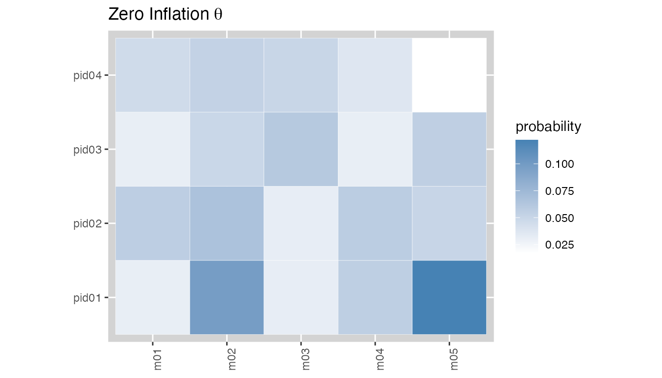
plot(fit, type = "beta")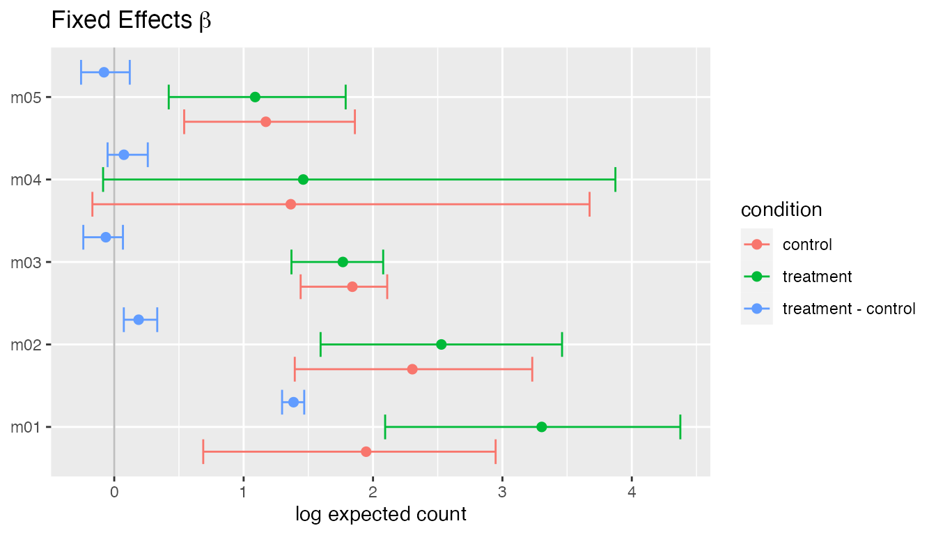
plot_pairs(fit, "m01", "m02", "m03")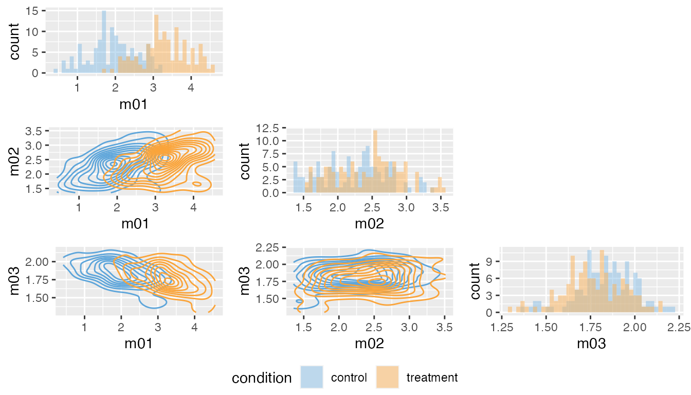
plot(fit, type = "sigma")
#> New names:
#> • `` -> `...1`
#> • `` -> `...2`
#> • `` -> `...3`
#> • `` -> `...4`
#> • `` -> `...5`
#> • `` -> `...6`
#> • `` -> `...7`
#> • `` -> `...8`
#> • `` -> `...9`
#> • `` -> `...10`
#> • `` -> `...11`
#> • `` -> `...12`
#> • `` -> `...13`
#> • `` -> `...14`
#> • `` -> `...15`
#> • `` -> `...16`
#> • `` -> `...17`
#> • `` -> `...18`
#> • `` -> `...19`
#> • `` -> `...20`
#> • `` -> `...21`
#> • `` -> `...22`
#> • `` -> `...23`
#> • `` -> `...24`
#> • `` -> `...25`
#> • `` -> `...26`
#> • `` -> `...27`
#> • `` -> `...28`
#> • `` -> `...29`
#> • `` -> `...30`
#> • `` -> `...31`
#> • `` -> `...32`
#> • `` -> `...33`
#> • `` -> `...34`
#> • `` -> `...35`
#> • `` -> `...36`
#> • `` -> `...37`
#> • `` -> `...38`
#> • `` -> `...39`
#> • `` -> `...40`
#> • `` -> `...41`
#> • `` -> `...42`
#> • `` -> `...43`
#> • `` -> `...44`
#> • `` -> `...45`
#> • `` -> `...46`
#> • `` -> `...47`
#> • `` -> `...48`
#> • `` -> `...49`
#> • `` -> `...50`
#> • `` -> `...51`
#> • `` -> `...52`
#> • `` -> `...53`
#> • `` -> `...54`
#> • `` -> `...55`
#> • `` -> `...56`
#> • `` -> `...57`
#> • `` -> `...58`
#> • `` -> `...59`
#> • `` -> `...60`
#> • `` -> `...61`
#> • `` -> `...62`
#> • `` -> `...63`
#> • `` -> `...64`
#> • `` -> `...65`
#> • `` -> `...66`
#> • `` -> `...67`
#> • `` -> `...68`
#> • `` -> `...69`
#> • `` -> `...70`
#> • `` -> `...71`
#> • `` -> `...72`
#> • `` -> `...73`
#> • `` -> `...74`
#> • `` -> `...75`
#> • `` -> `...76`
#> • `` -> `...77`
#> • `` -> `...78`
#> • `` -> `...79`
#> • `` -> `...80`
#> • `` -> `...81`
#> • `` -> `...82`
#> • `` -> `...83`
#> • `` -> `...84`
#> • `` -> `...85`
#> • `` -> `...86`
#> • `` -> `...87`
#> • `` -> `...88`
#> • `` -> `...89`
#> • `` -> `...90`
#> • `` -> `...91`
#> • `` -> `...92`
#> • `` -> `...93`
#> • `` -> `...94`
#> • `` -> `...95`
#> • `` -> `...96`
#> • `` -> `...97`
#> • `` -> `...98`
#> • `` -> `...99`
#> • `` -> `...100`
#> • `` -> `...101`
#> • `` -> `...102`
#> • `` -> `...103`
#> • `` -> `...104`
#> • `` -> `...105`
#> • `` -> `...106`
#> • `` -> `...107`
#> • `` -> `...108`
#> • `` -> `...109`
#> • `` -> `...110`
#> • `` -> `...111`
#> • `` -> `...112`
#> • `` -> `...113`
#> • `` -> `...114`
#> • `` -> `...115`
#> • `` -> `...116`
#> • `` -> `...117`
#> • `` -> `...118`
#> • `` -> `...119`
#> • `` -> `...120`
#> • `` -> `...121`
#> • `` -> `...122`
#> • `` -> `...123`
#> • `` -> `...124`
#> • `` -> `...125`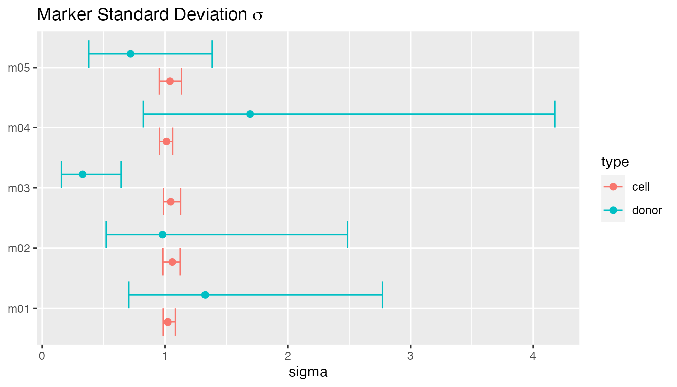
plot(fit, type = "Cor")
#> [[1]]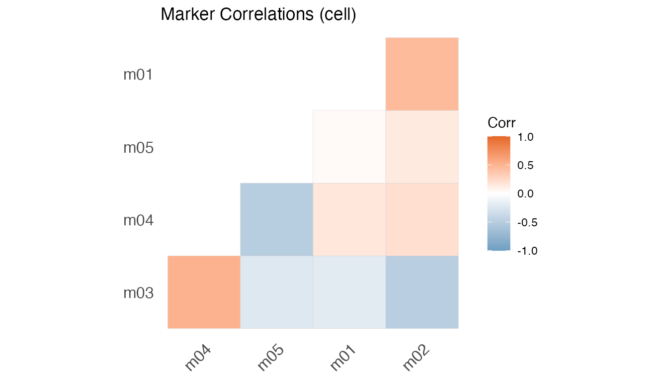
#>
#> [[2]]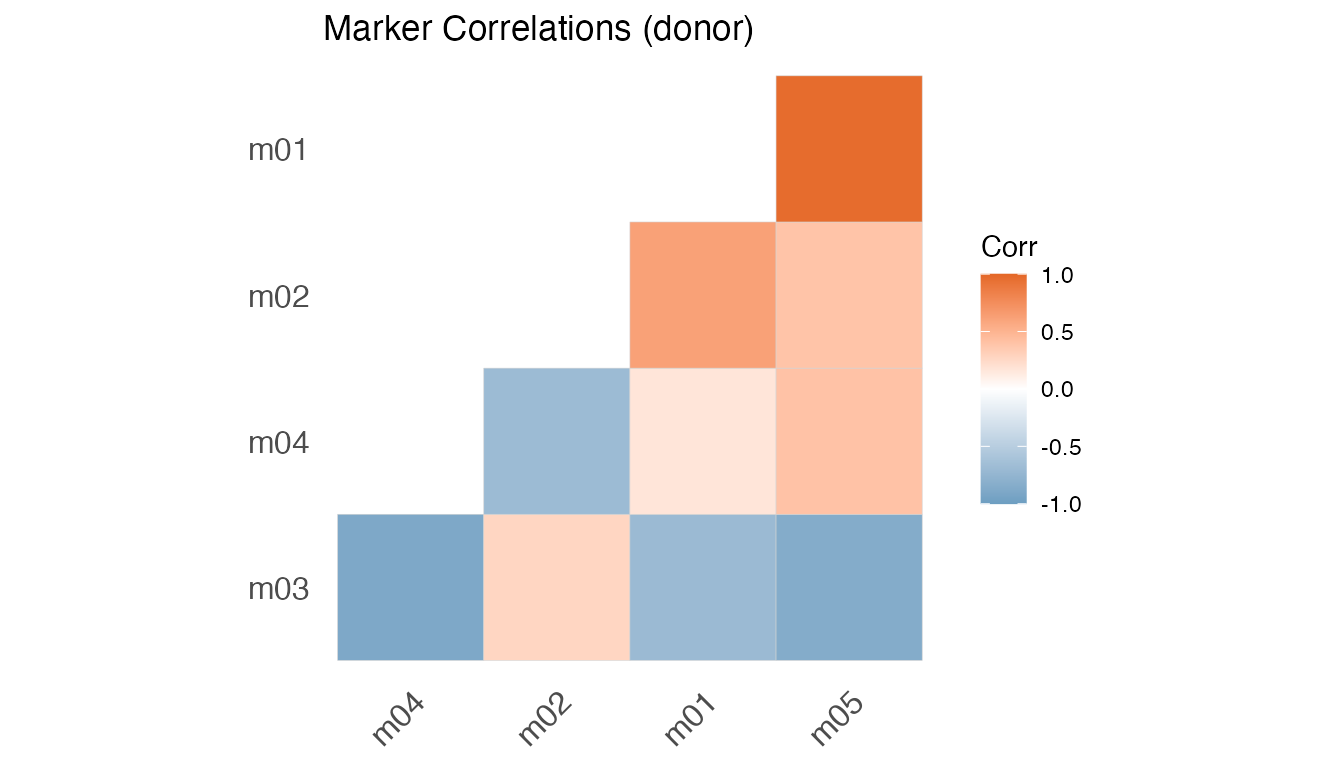
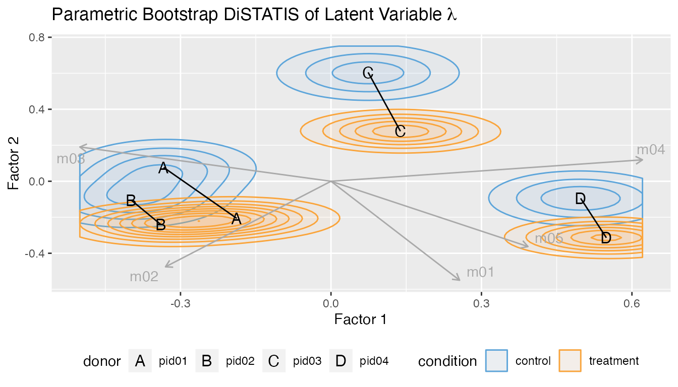
Multivariate DiSTATIS plot.
plot_distatis(fit, ndraws = 125)
#> Warning: The `.dots` argument of `group_by()` is deprecated as of dplyr 1.0.0.
#> ℹ The deprecated feature was likely used in the dplyr package.
#>   Please report the issue at <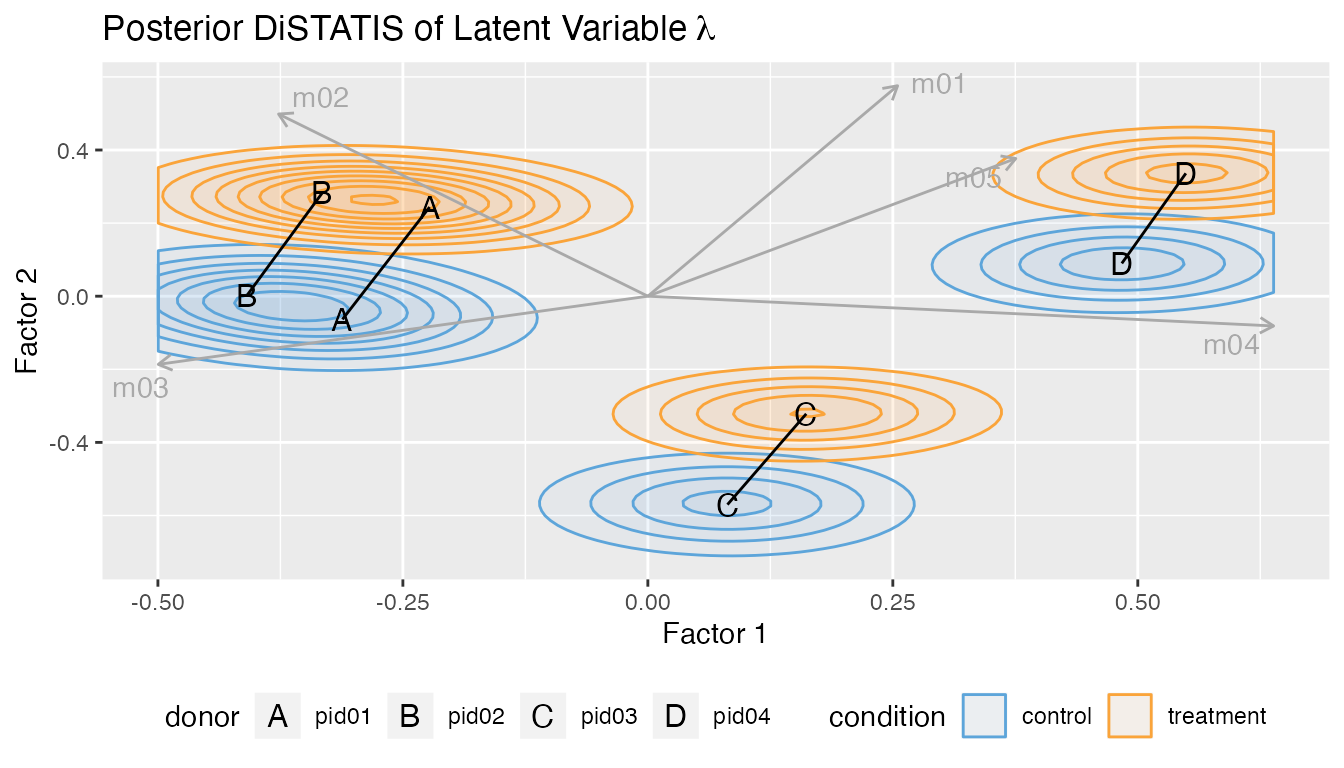
Frequentist Inference
Fit model using composite maximum likelihood estimatation.
fit = poisson_lognormal_mcle(df,
                             protein_names = protein_names,
                             condition = condition,
                             group = group,
                             ncores = 1)
Plot marginal credible intervals.
plot(fit, type = "beta")
#> New names:
#> • `` -> `...1`
#> • `` -> `...2`
#> • `` -> `...3`
#> • `` -> `...4`
#> • `` -> `...5`
#> • `` -> `...6`
#> • `` -> `...7`
#> • `` -> `...8`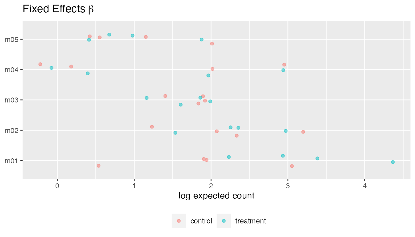
plot(fit, type = "sigma")
#> New names:
#> • `` -> `...1`
#> • `` -> `...2`
#> • `` -> `...3`
#> • `` -> `...4`
#> • `` -> `...5`
#> • `` -> `...6`
#> • `` -> `...7`
#> • `` -> `...8`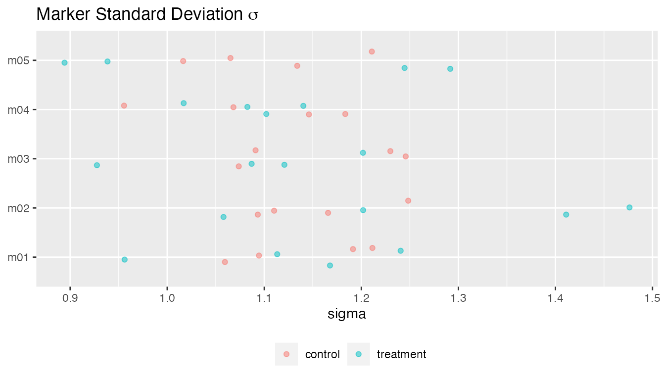
plot(fit, type = "Cor")
Multivariate DiSTATIS plot.
plot_distatis(fit, ndraws = 125)